Sync: Aligning with Edges

Document organization:

General principles
Needed components and their use
Worked example showing command line parameters
Plug for scripted pipeline

Overview

Definition: SpikeGLX Data Stream = Set of channels sampled according to a given sample clock.

Examples of streams:

Neuropixels probe. The sample clock lives in the headstage. The AP-band data are acquired at nominally 30kHz but actual rates may differ by as much as one Hz. If that probe acquires a separate LF-band, the same clock is used and the LF-band sample rate is exactly 1/12 that of the AP-band. In short each probe, really each headstage, is a separate stream.
Onebox ADC channels: An imec Onebox can record from several probes, each of which is a stream, and it can record several analog and digital non-neural channels at ~30kHz, which we also regard as a stream. This gets its own obx file type.
NI device: You can use a NI multifunction/multichannel device to record your non-neural analog and digital (TTL) channels. You'll have several options for setting its sample rate. This is one stream.

Actually SpikeGLX lets you run two NI devices of the same model together, one master and one slave, so that they share a common clock, and are thus recorded and treated as a single stream with double the channel capacity.

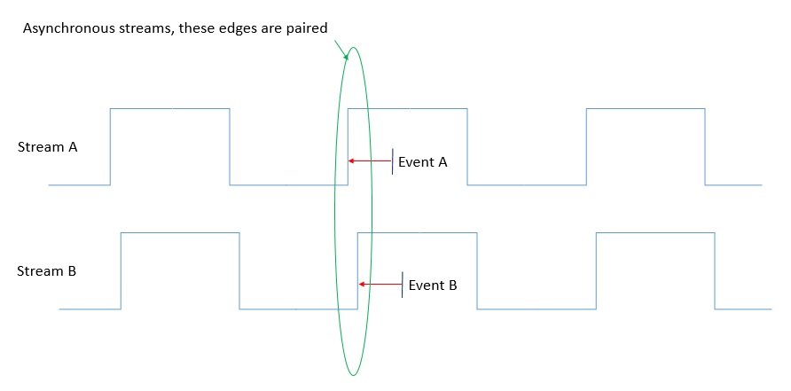
Problem: Generally, data streams each have their own clock, hence, their own nominal sample rate, and run asynchronously. Moreover, sample clock rates will vary with temperature. This makes it necessary and challenging to synchronize (align) events acquired in different streams.

Solution: SpikeGLX (plus companion tools CatGT and TPrime) provide a reliable means of aligning data to sub-millisecond accuracy. Note that the SpikeGLX "alignment" process does not entail any resampling or editing of the raw acquired data. Rather it is a scheme for mapping post-analysis event times (seconds, not samples) from one coordinate system to another.

This mapping scheme is implemented as follows. A common 1 Hz square wave is recorded in one channel of each data stream throughout the experiment. In offline processing, the rising edges in this "sync wave" are paired across streams A & B. Any event (T) occurring in B is no more than one second away from a nearest (preceding) sync wave edge (Eb) in stream B. That edge has a simultaneously occurring matching edge (Ea) in stream A. To map T in stream B to T' in stream A, we simply calculate:

    T' = T - Eb + Ea.

<BR/>

Assuming we can correctly pair sync wave edges, the error on any mapped time is bounded by [1s * rate_error/rate]. For example, if the nominal probe sample rate is 30kHz and the error in that value is 3Hz, then the error in the mapped time would be 0.1ms.

Rate error arises when we do not know the actual clock rate. The two largest sources of error are (1) bad/unknown calibration (the largest difference from 30kHz we've seen post calibration is 1Hz), and (2) temperature variation, which we measure to be very small near room temperature: < 0.01Hz/5C. So mapping errors after application of TPrime are typically smaller than 0.1ms.

Briefly, the sync-related roles of various components are the following, listed in the order you would organize your workflow:

SpikeGLX:
- Calibrate sample rates
- Recalibrate rates from run
- Generate and record runtime sync wave
CatGT:
- Extract tables of sync wave edges
- Extract tables of non-neural event times
Your_favorite_spike_sorter:
- Extract tables of spike times
TPrime:
- Remap all tables of times to reference stream coordinates

The remaining sections cover some how-to tips.

SpikeGLX: Clock calibration

Do I need it?

Calibrating your clocks is useful for these reasons:

It's a test of headstage health. The measured rate shouldn't be more than 1Hz different than 30kHz, and if you repeat the measurement, it should remain stable to < 0.1Hz.
TPrime should also be used if you plan to publish claims about timing. But if you are just browsing in the FileViewer or eyeballing PSTH plots to roughly see how things line up without the bother of running TPrime, that will work better if all clocks are at least calibrated.
TPrime needs to be able to identify pairs of matching edges. If the recorded times of edges in the sync wave are a second or more off, the adjustment may suffer phase error. This could be a problem in a long run where error is cumulative. To estimate the duration, consider that an uncalibrated clock could run as much as 1Hz differently than 30kHz. Then a problem will occur at time T, where 1Hz * T = 30000 or T = 8.3 hours.

How to

Using the Sync tab in the Configuration dialog, you:

select a sync wave source
specify for each stream which channels are getting sync wave input
check Use next run for calibration (and select a run-length)

This configures a special purpose run and does a post-run analysis to count how many samples are actually occurring between edges of the sync wave, and thereby deduces the true sample rate. It reports its results in a dialog for you to accept or reject. If accepted these become saved in a database and are used for subsequent runs of those hardware devices until you decide to do another calibration.

Tips

You probably don't need to calibrate a given device more than once, but you might as well get a good measurement for that one time. We recommend setting the calibration data collection time to 40 min.

SpikeGLX: Recalibration

Conditions

Even if you never calibrated your sample clocks before, you can still calibrate them after the fact from existing run data if:

You were recording the sync wave in each stream you want to calibrate.
The run is long enough to get a reasonable estimate, at least 20 min.

How to

To do this, choose item Sample Rates From Run from the Tools menu and follow the instructions in the dialog. As with a first-time calibration it will show you results that you can accept or not. If you accept you can further choose whether to edit this run's metadata, and whether to update the database and use the new rates going forward.

The dialog won't let you select imec LF-band files because their time resolution is too low. Rather, select the partner AP-band file. Both AP and LF metadata will be updated together. Note that the LF rate is exactly 1/12 the AP rate.

SpikeGLX: Run with sync

How to

It's easy to do a run that records the sync waveform.

Specify a source/generator of the common sync waveform. You have several options:
- Select any one of the imec slots.
- Select your NI multifunction I/O device (SpikeGLX programs its output).
- Use your own signal generator. Set it for 1 Hz and 50% duty cycle.
Feed wires from the source to one channel in each stream.
- For the PXI based versions, all of the imec modules share the sync signal using the chassis backplane, so only one slot (module) needs a wire connected to its SMA connector, whether it is specified as input or output (source). So you connect a wire to just one (active) module, and all imec probes will automatically record the sync wave.
- If NI is the source, the Notes field indicates which output terminal to connect.
Tell the Sync tab which channels you wired so SpikeGLX can locate the waveform in each stream.
- For NP 1.0 and later, this signal is hard wired to appear on bit #6 of the last 16-bit word in the stream, the SY channel.

File T-zero and length

When you are running with sync enabled on the Sync tab, whenever a file-writing trigger event occurs and a new set of files is started, SpikeGLX internally uses the edges to make sure that the files all start at a common wall time. Each file's metadata records the sample index number of the first sample in that file: firstSample. These samples are aligned to each other. Said another way, the files share a common T0.

While long files are being written, their alignment may slowly degrade because they are running and recording according to their own clock rates. If the clocks have been calibrated this drift will be a bit smaller, but nothing happens during writing to "reset" the alignment. Doing that would entail interpolating or resampling of data, which we do not do. (Note that TPrime corrects times by referencing times to sync edges no matter how long the file is. It's effectively like getting periodic resets throughout the run.)

The writing phase for a given set of files (given g, t index) ends when a stop event occurs. Perhaps a writing timer elapses, or a TTL trigger gets a stop signal, or you click the Disable or Stop button. Any such event stops all the streams and closes the files, but the "right-hand-side" or "trailing edges" of the files are not guaranteed to be perfectly aligned. The files are often quite close to being the same length (metadata item fileTimeSecs), but this is not controlled.

CatGT: Event extraction

CatGT can perform several post-processing jobs, singly or in combination:

Concatenate a g/t-series of separate trial files (whence the name).
Apply tshift, band-pass and CAR filters to neural channels.
Edit out saturation artifacts.
Extract tables of sync waveform edge times to drive TPrime.
Extract tables of any other TTL event times to be aligned with spikes.

The extraction features are discussed here.

General

Starting with version 3.0, CatGT extracts sync edges from all streams by default, unless you specify the -no_auto_sync option (see below).

There are five extractors for scanning and decoding nonneural data channels in any data stream. They differ in the data types they operate upon:

xa: Finds positive pulses in any analog channel.
xd: Finds positive pulses in any digital channel.
xia: Finds inverted pulses in any analog channel.
xid: Finds inverted pulses in any digital channel.
bf: Decodes positive bitfields in any digital channel.

The first three parameters of any extractor specify the stream-type, stream-index and channel (16-bit word) to operate on, E.g.:

-xa=js,ip,word, <additional parameters>

Extractors js (stream-type):

NI: js = 0 (any extractor).
OB: js = 1 (any extractor).
AP: js = 2 (only {xd, xid} are legal).

Extractors do not work on LF files.

Extractors ip (stream-index)

NI: ip = 0 (there is only one NI stream).
OB: ip = 0 selects obx0, ip = 7 selects obx7, etc.
AP: ip = 0 selects imec0, ip = 7 selects imec7, etc.

Extractors word

Word is a zero-based channel index. It selects the 16-bit data word to process.

word = -1, selects the last word in that stream. That's especially useful to specify the SY word at the end of a Onebox or probe stream.

It may be helpful to review the organization of words and bits in data streams in the SpikeGLX User Manual.

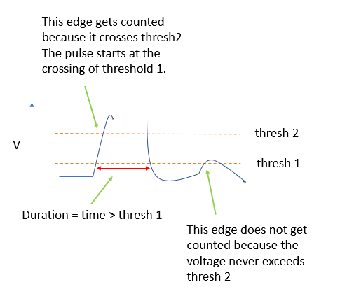
Extractors positive pulse

starts at low non-negative baseline (below threshold)
has a leading/rising edge (crosses above threshold)
(optionally) stays high/deflected for a given duration
has a trailing/falling edge (crosses below threshold)

The positive pulse extractors {xa, xd} make text files that report the times (seconds) of the leading edges of matched pulses.

Extractors xa

Following -xa=js,ip,word, these parameters are required:

Primary threshold-1 (V).
Optional more stringent threshold-2 (V).
Milliseconds duration.

If your signal looks like clean square pulses, set threshold-2 to be closer to baseline than threshold-1 to ignore the threshold-2 level and run more efficiently. For noisy signals or for non-square pulses set threshold-2 to be farther from baseline than theshold-1 to ensure pulses attain a desired deflection amplitude. Using two separate threshold levels allows detecting the earliest time that pulse departs from baseline (threshold-1) and separately testing that the deflection is great enough to be considered a real event and not noise (threshold-2).

Extractors xd

Following -xd=js,ip,word, these parameters are required:

Index of the bit in the word.
Milliseconds duration.

Extractors both xa and xd

All indexing is zero-based.
Milliseconds duration means the signal must remain deflected from baseline for that long.
Milliseconds duration can be zero to specify detection of all leading edges regardless of pulse duration.
Milliseconds duration default precision (tolerance) is +/- 20%.
- Default tolerance can be overridden by appending it in milliseconds as the last parameter for that extractor.
- Each extractor can have its own tolerance.
- E.g. -xd=js,ip,word,bit,100 seeks pulses with duration in default range [80,120] ms.
- E.g. -xd=js,ip,word,bit,100,2 seeks pulses with duration in specified range [98,102] ms.
A given channel or even bit could encode two or more types of pulse that have different durations, E.g. -xd=0,0,8,0,10 -xd=0,0,8,0,20 scans and reports both 10 and 20 ms pulses on the same line.
Each option, say -xd=2,0,384,6,500, creates an output file whose name reflects the parameters, e.g., run_name_g0_tcat.imec0.ap.xd_384_6_500.txt.
The threshold is not encoded in the -xa filename; just word and milliseconds.
The run_name_g0_fyi.txt file lists the full paths of all generated extraction files.
The files report the times (s) of leading edges of detected pulses; one time per line, \n line endings.
The time is relative to the start of the stream in which the pulse is detected (native time).

Extractors inverted pulse

starts at high positive baseline (above threshold)
has a leading/falling edge (crosses below threshold)
(optionally) stays low/deflected for a given duration
has a trailing/rising edge (crosses above threshold)

Although the shape is "inverted," these pulses are nevertheless entirely non-negative.

The inverted pulse extractors {xia, xid} make text files that report the times (seconds) of the leading edges of matched pulses.

The inverted pulse versions work exactly the same way as their positive counterparts. Just keep in mind that inverted pulses have a high baseline level and deflect toward lower values.

Extractors bf (bit-field)

The -xd and -xid options treat each bit of a digital word as an individual line. In contrast, the -bf option interprets a contiguous group of bits as a non-negative n-bit binary number. The -bf extractor reports value transitions: the newest value and the time it changed, in two separate files. Following -xa=js,ip,word, the parameters are:

startbit: lowest order bit included in group (range [0..15]),
nbits: how many bits belong to group (range [1..<16-startbit>]).
inarow: a real value has to persist this many samples in a row (1 or higher).

In the following examples we set inarow=3:

To interpret all 16 bits of NI word 5 as a number, set -bf=0,0,5,0,16,3.
To interpret the high-byte as a number, set -bf=0,0,5,8,8,3.
To interpret bits {3,4,5,6} as a four-bit value, set -bf=0,0,5,3,4,3.

You can specify multiple -bf options on the same command line. The words and bits can overlap.

Each -bf option generates two output files, named according to the parameters (excluding inarow), for example:

run_name_g0_tcat.nidq.bfv_5_3_4.txt.
run_name_g0_tcat.nidq.bft_5_3_4.txt,

The two files have paired entries. The bfv file contains the decoded values, and the bft file contains the time (seconds from file start) that the field switched to that value.

Extractors no_auto_sync option

Starting with version 3.0, CatGT automatically extracts sync edges from all streams unless you turn that off using -no_auto_sync.

For an NI stream, CatGT reads the metadata to see which analog or digital word contains the sync waveform and builds the corresponding extractor for you, either -xa=0,0,word,thresh,0,500 or -xd=0,0,word,bit,500.

For OB and AP streams, CatGT seeks edges in bit #6 of the SY word, as if you had specified -xd=1,ip,-1,6,500 and/or -xd=2,ip,-1,6,500.

TPrime: Remapping

General

After recording, spike sorting, TTL extraction...Now you need to convert all these times from the native timelines of the data streams in which they were measured to a common reference timeline. That's the only way you can compare them! That's what TPrime does.

TPrime uses three types of files:

tostream: The reference stream we will map to. It is defined by a file of sync wave edges as extracted by CatGT. There is only one of these.
fromstream: A native stream we will map from. There can be several of these. A fromstream is identified by a file of sync wave edges extracted by CatGT, and, an arbitrary positive integer that is a shorthand for that stream, just so you don't have to type the edge-file-path over and over.
events file: These are times you want to convert. Typically you will have a different file for every event class, such as all the spikes from probe zero, or all the nose_poke times from the NI stream. On the command line for each such file you will specify the stream index for the matching fromstream, an input file of native times, a new file path for the output times.

Events files

Key specs for events files:

Input and output file type can be .txt or .npy (Kilosort).
You can mix types: txt in, npy out, etc.
Times are seconds, they are not sample numbers.
Times are relative to the start of the file.
Times are in ascending order.

Worked example

Outline

Here we'll show actual command lines for CatGT and TPrime. We'll use a very simple contrived experiment for concreteness.

Two probes {0,1}.
Two non-neural NI signals {go_cue, nose_poke}.

SpikeGLX settings

We focus here on SpikeGLX settings relevant to the CatGT/TPrime command lines...

Imec Setup tab:
- (probe 0) :: Save chans: 0-49,200-249,768 ; 2 blocks of 50 channels + SY
- (probe 1) :: Save chans: all
NI Setup tab:
- Primary device :: XA box: 0 ; go_cue as analog just to demonstrate
- Primary device :: XD box: 2,3 ; 2=nose_poke, 3=sync
- Common analog :: AI range: -5, 5
- Maps :: Channels to save: all
Sync tab:
- Square wave source :: Imec slot 3
- Inputs :: Nidq: Digital bit, 3
Triggers tab
- Trigger mode: Immediate start ; single file, record upon button press
Save tab:
- Run naming :: Data directory :: D:/Data
- Run naming :: Run name: demo
- Run naming :: Folder per probe: checked

SpikeGLX output

D:/data/                                ; data folder
    demo/                               ; run folder
        demo_g0_imec0/                  ; probe folder
            demo_g0_t0.imec0.ap.bin
            demo_g0_t0.imec0.ap.meta
            demo_g0_t0.imec0.lf.bin
            demo_g0_t0.imec0.lf.meta
        demo_g0_imec1/                  ; probe folder
            demo_g0_t0.imec1.ap.bin
            demo_g0_t0.imec1.ap.meta
            demo_g0_t0.imec1.lf.bin
            demo_g0_t0.imec1.lf.meta
        demo_g0_t0.nidq.bin             ; ni at top of run folder
        demo_g0_t0.nidq.meta

CatGT command line

I broke the line into several groups using continuation characters (^) but doing so is aesthetic only. The comments (;) must not appear in real commands.

IMPORTANT: In real command lines there should be NO extra spaces inserted into the text of options, NOR following a caret (^) character.

> CatGT ^
 -dir=D:/data -run=demo -prb_fld ^      ; run naming
 -g=0 -t=0,0 ^                          ; g and t range
 -ap -prb=0,1 -ni ^                     ; which streams
 -apfilter=butter,12,300,9000 ^         ; filters
 -xa=0,0,0,1.1,0,25 ^                   ; go_cue = 25 ms square pulse
 -xd=0,0,1,2,0 ^                        ; nose_poke duration unknown
 -dest=D:/CGT_OUT ^                     ; let's put output in new place
 -out_prb_fld                           ; and use an output folder per probe

CatGT output

D:/CGT_OUT/                                        ; master output folder
    catgt_demo_g0/                                 ; run output folder
        demo_g0_imec0/                             ; probe folder
            demo_g0_tcat.imec0.ap.bin              ; filtered data for KS2
            demo_g0_tcat.imec0.ap.meta
            demo_g0_tcat.imec0.ap.xd_100_6_500.txt ; sync edges
        demo_g0_imec1/                             ; probe folder
            demo_g0_tcat.imec1.ap.bin              ; filtered data for KS2
            demo_g0_tcat.imec1.ap.meta
            demo_g0_tcat.imec1.ap.xd_384_6_500.txt ; sync edges
        demo_g0_tcat.nidq.xa_0_25.txt              ; go_cue
        demo_g0_tcat.nidq.xd_1_2_0.txt             ; nose_poke
        demo_g0_tcat.nidq.xd_1_3_500.txt           ; sync edges

Kilosort 2 output

Suppose we tell KS2 to put its output into the same folders as the CatGT output. Of course we run KS2 once for each probe. The output from KS2 is then:

D:/CGT_OUT/                                 ; master output folder
    catgt_demo_g0/                          ; run output folder
        demo_g0_imec0/                      ; probe folder
            amplitudes.npy
            channel_map.npy
            ...
            spike_times.npy                 ; this is in samples
            ...
            whitening_mat_inv.npy
        demo_g0_imec1/                      ; probe folder
            amplitudes.npy
            channel_map.npy
            ...
            spike_times.npy                 ; this is in samples
            ...
            whitening_mat_inv.npy

Samples to times

Most spike sorters report spike times as sample indices so we'll need our own mini program to convert those to times in seconds. The program:

Loads array spike_times.npy.
Parses value imSampRate from the metadata file.
Divides the rate into each array element.
Writes the times out in same folder as spike_seconds.npy.

Metadata parsers are available here.

IMPORTANT: npy files usually store the values as doubles which preserves full numeric precision. Whenever you are saving clock rates or event times as text, be sure to write the values to microsecond-level precision. Keep six digits in the fractional part.

TPrime command line

Let's map all times to probe-0:

> TPrime -syncperiod=1.0 ^
 -tostream=D:/CGT_OUT/catgt_demo_g0/demo_g0_imec0/demo_g0_tcat.imec0.ap.xd_100_6_500.txt ^
 -fromstream=1,D:/CGT_OUT/catgt_demo_g0/demo_g0_imec1/demo_g0_tcat.imec1.ap.xd_384_6_500.txt ^
 -fromstream=2,D:/CGT_OUT/catgt_demo_g0/demo_g0_tcat.nidq.xd_1_3_500.txt ^
 -events=1,D:/CGT_OUT/catgt_demo_g0/demo_g0_imec1/spike_seconds.npy,D:/CGT_OUT/catgt_demo_g0/demo_g0_imec1/spike_seconds_adj.npy ^
 -events=2,D:/CGT_OUT/catgt_demo_g0/demo_g0_tcat.nidq.xa_0_25.txt,D:/CGT_OUT/catgt_demo_g0/go_cue.txt ^
 -events=2,D:/CGT_OUT/catgt_demo_g0/demo_g0_tcat.nidq.xd_1_2_0.txt,D:/CGT_OUT/catgt_demo_g0/nose_poke.txt

Scripted pipeline

It can be daunting to get all these command lines correct. You might want to check out Jennifer Colonell's version of the Allen Institute ecephys_spike_sorting pipeline. This Python script-driven pipeline chains together: CatGT, KS2, Noise Cluster Tagging, C_Waves, QC metrics, TPrime. It's been tested a lot here at Janelia and several other institutions.

fin

Keys	Action
`?`	Open this help
`n`	Next page
`p`	Previous page
`s`	Search